Classification: Decision Trees, Naive Bayes & Gaussian Bayes Classifier

Classification is a type of supervised learning. It specifies the class to which data elements belong to and is best used when the output has finite and discrete values. It predicts a class for an input variable as well.

There are two types of Classification:

Binomial: This is a type of classification where algorithms divide the data into two classes. We fed the data into algorithms after training the algorithms it forms two classes thus passing a new data it classifies the data into either of the two classes. A simple example of this type of classification algorithms is linear regression.
Multi-Class: This is a type of classification where algorithms divide’s the data into multi classes according to the types of regions formed. By the term, a region formed it means, when the data will be visualised there would be several regions where different data would be close to each other and the new data provided to it would be classified based on the position of the data nearer to the regions. A fundamental example of this type of algorithms is Decision trees.

Use Cases: In today’s world classification algorithms are used very extensively, there is a very wide userbase for classification. You may also have someday used them without knowing actual implementation.

Some of the key areas where classification cases are being used which you can easily relate to are:

Dividing information by buy history
Identifying diverse action types in movement sensors
To find whether an email received is spam
Identify customer segments
Find if a bank loan is granted
Simply by knowing the pass mark, a hyperplane can be drawn. Suppose 40 is the pass mark a hyperplane can be drawn any student above 40 is classified as pass and below 40 classified as a fail.
Classifying words as nouns, pronouns and verbs

Types of Classification Algorithms:

Let’s have a quick look into the types of Classification Algorithm below.

Linear Models
Logistic Regression
Support Vector Machines
Non-linear models
K-nearest Neighbors (KNN)
Kernel Support Vector Machines (SVM)
Naïve Bayes
Decision Tree Classification
Random Forest Classification
Gaussian Naive Bayes

Steps requires to build a classifier:

Initialise: Model the classifier to be used
Train: Train the classifier using a good training data
Predict: Pass on to a new data X to the model that evaluates the data to predict(X)
Evaluate: Evaluate the model

Decision Trees: Decision Tree is a simple tree like structure, model makes a decision at every node. The paths from root to leaf represent classification rules. At every node one has to take the decision as to travel through which path to get to a leaf node. That decisions at every node are dependent on the features/columns of the training set or the content of the data. It is very useful in simple tasks where by a simple logic one can understand where to classify things. One of the most popular algorithm cause of its simplicity and its usefulness, it is quite easy to explain to client and easy to show how a decision process works!

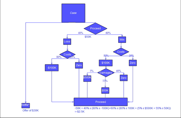
A decision tree consists of three types of nodes:

Decision Nodes: Typically represented by squares
Chance Nodes: Typically represented by circles
End Nodes: Typically represented by triangles

Why decision trees are popular?

Easy to interpret and present
Well defined Logic, mimic human level thought
Random Forests, ensembles of decision trees are more powerful classifiers
Feature values are preferred to be categorical. If the values are continuous then they are discretised prior to building the model

Build Decision Trees:

Two common algorithms:

CART (Classification and Regression Trees) → uses Gini Index(Classification) as a metric
ID3 (Iterative Dichotomiser 3) → uses Entropy function and Information gain as metrics

Decision tree using flow chart symbol

Implementation

Using the sklearn library we can easily implement Decision Tree. Also, with help from Graphviz we could also easily visualise them.

from sklearn.tree import DecisionTreeClassifier
from sklearn.tree import DecisionTreeClassifier
from sklearn.tree import DecisionTreeClassifier
sk_tree.fit(train_data[input_cols],train_data[output_cols])
sk_tree.score(test_data[input_cols],test_data[output_cols])

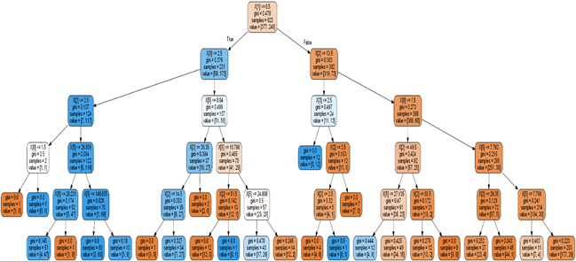
Visualisation of a Decision Tree:

import pydotplus
from sklearn.externals.six import StringIO
from IPython.display import Image
from sklearn.tree import export_graphviz
dot_data = StringIO()
export_graphviz(sk_tree,out_file=dot_data,filled=True,rounded=True)
graph = pydotplus.graph_from_dot_data(dot_data.getvalue())
Image(graph.create_png())

Disadvantages

A decision tree can create complex trees that do not generalise well, and decision trees can be unstable because small variations in the data might result in a completely different tree being generated.

Naive Bayes: This algorithm based on Bayes’ theorem with the assumption of independence between every pair of features. In simple terms, a Naive Bayes classifier assumes that the presence of a particular feature in a class is unrelated to the presence of any other feature. For example, a fruit may be considered to be orange if it is orange in colour, round, and about three inches in diameter.

Even if these features depend on each other or upon the existence of the other features, all of these properties independently contribute to the probability that this fruit is an orange and that is why it is known as ‘Naive’. This algorithm requires a small amount of training data to estimate the necessary parameters. Naive Bayes classifiers are extremely fast compared to more sophisticated methods. Naive Bayes model is easy to build and particularly useful for very large data sets.

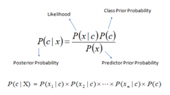
Above,

P(c|x) is the posterior probability of class (c, target) given predictor (x, attributes)
P(c) is the prior probability of class
P(x|c) is the likelihood which is the probability of predictor given class
P(x) is the prior probability of predictor

Relationships/Formulas

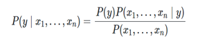
Naive Bayes methods are a set of supervised learning algorithms based on applying Bayes’ theorem with the “naive” assumption of conditional independence between every pair of features given the value of the class variable. Bayes’ theorem states the following relationship, given class variable y and dependent feature vector through:

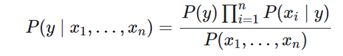
Using conditional assumption:

for all, this relationship is simplified to:

Since is constant given the input, we can use the following classification rule:

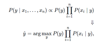
and we can use Maximum A Posteriori (MAP) estimation to estimate P(y) and P(∣y); the former is then the relative frequency of class y in the training set.

Why Naïve Bayes’?

Naive Bayes Classifier and Collaborative Filtering together create a recommendation system that together can filter very useful information that can provide a very good recommendation to the user.
It is widely used in a spam filter, it is widely used in text classification due to a higher success rate in multinomial classification with an independent rule.
Used widely for multiclass classification.
As Naïve Bayes’ is very fast thus this is also widely used for real-time classification.

Disadvantage

Sometimes it can be a bad estimator.

Types of Naïve Bayes’ models

Gaussian Naïve Bayes’
Multinomial Naïve Bayes’
Complement Naïve Bayes’
Bernoulli Naïve Bayes’
Categorical Naïve Bayes’

There are three types of Naive Bayes model under the scikit-learn library:

Gaussian
Multinomial
Bernoulli

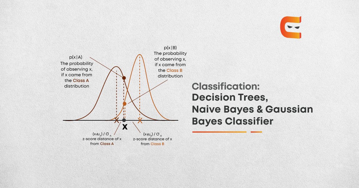
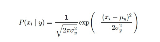
Gaussian Naive Bayes: Naive Bayes can be extended to real-valued attributes, most commonly by assuming a Gaussian distribution. This extension of naive Bayes is called Gaussian Naive Bayes. Other functions can be used to estimate the distribution of the data, but the Gaussian (or Normal distribution) is the easiest to work with because you only need to estimate the mean and the standard deviation from your training data. When working with continuous data, an assumption often taken is that the continuous values associated with each class are distributed according to a normal (or Gaussian) distribution. The likelihood of the features is assumed to be as below:

Sometimes assume variance:

Is independent of Y (i.e., σi),
Or independent of Xi (i.e., σk)
Or both (i.e., σ)

An approach to create a simple model is to assume that the data is described by a Gaussian distribution (also called Normal Distribution) with no co-variance (independent dimensions) between dimensions. This model can be fit by simply finding the mean and standard deviation of the points within each label, which is all what is needed to define such a distribution.

Implementation:

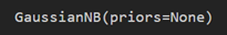
from sklearn.naive_bayes import GaussianNB
from sklearn.naive_bayes import GaussianNB
from sklearn.datasets import make_classification
import matplotlib.pyplot as plt
X,Y = make_classification(n_samples=200, n_features=2 , n_informative=2, n_redundant=0, random_state=4)
plt.scatter(X[:,0],X[:,1],c=Y)
plt.show()

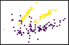
Here, we could easily see this algorithm works very well.

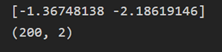
print(X[0])
print(X.shape) #Continuous Value Features

# Train our classifier
gnb.fit(X,Y)

gnb.score(X,Y)

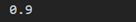
Here 0.9 means 90% of accuracy. You could easily see that by writing such a simple implementation with help of sklearn we could easily get that much of accuracy. You can also get the glimpse of the output ypred.

ypred = gnb.predict(X)
print(ypred)

For better summarising the result y is printed below.

print(Y)

Summary

From the start, we can conclude that we get to know about Classification Algorithms. Its use cases in real-world and why this algorithm is used widely. We saw types of classification and the types of classification algorithms. Just after this comes the Decision Tree with its logic and implementations using sklearn, we also visualised Decision tree to get a proper view. We also saw how fast is Naïve Bayes’ algorithms and its types and the major formulas. In the end, we implemented Gaussian Naïve Bayes’ which is an extension of Naïve Bayes. These algorithms with some of the others are very extensively used algorithms in day to day life. These algorithms are not only changing the world but also the way we visualise data.

To explore more about Machine Learning, read here.

By Tusshar Verma