Clustering in Machine Learning for Python

Introduction

Hey! Am I the only one who likes to watch Netflix and chill on weekends? Certainly not, but have you ever wondered how Netflix and Amazon Prime Videos provide you movie recommendations depending on your taste?

Seemingly, their recommendation system is intelligent. It strives to help us find the best web series or movies to watch with minimal effort by providing a list of trending ones every week or group them according to their popularity and genres like comedy, horror, or thriller.

Well, all these streaming services that offer a wide variety of award-winning television shows, movies, documentaries, etc., use a revolutionary technology known as  – “Machine Learning.”

That sounds interesting, right?

Image Source: www.netflix.com

From the above picture, we can see that the shows or movies are recommended based on our history.

In this blog, we will discuss the basics of machine learning and see its types. We will then jump to look at the clustering in machine learning, which helps in recommendations. Towards the end of this blog, we will look at the advantages, disadvantages, and last but not least, its applications.

What is Machine Learning?

The formal definition is something like this:

“Machine Learning is the science of getting computers to learn and act like humans do, and improve their learning over time in autonomous fashion, by feeding them data and information in the form of observations and real-world interactions.”

Watch below what Ankush Singla, Co-Founder of Coding Ninjas has to say. 

But in simple terms, machine learning is a revolutionary technology that gives devices the ability to learn from their experiences and improve themself over time.

Now let’s move on to its type.

There are three types of Machine Learning:

• Supervised Learning
• Unsupervised Learning 
• Reinforcement Learning (Not discussed in this blog)

Supervised Learning

Supervised learning is the machine learning task of learning a function that maps an input to an output based on example input-output pairs. It infers a function from labeled training data consisting of a set of training examples. We can have a detailed blog on supervised learning in the future. Let’s just focus on clustering in machine learning from unsupervised learning.

Unsupervised Learning

The data you categorize into groups based on some patterns or correlations is called unsupervised learning. Clustering is one of the widely used techniques in unsupervised learning. We have multiple clustering in machine learning techniques and have algorithms designed to leverage these techniques, which we will cover later in this blog, so stay tuned folks!

Let’s first try to understand what a cluster means. According to ‘Cambridge Dictionary,’ a cluster means – a group of similar things that are close together, sometimes surrounding something.

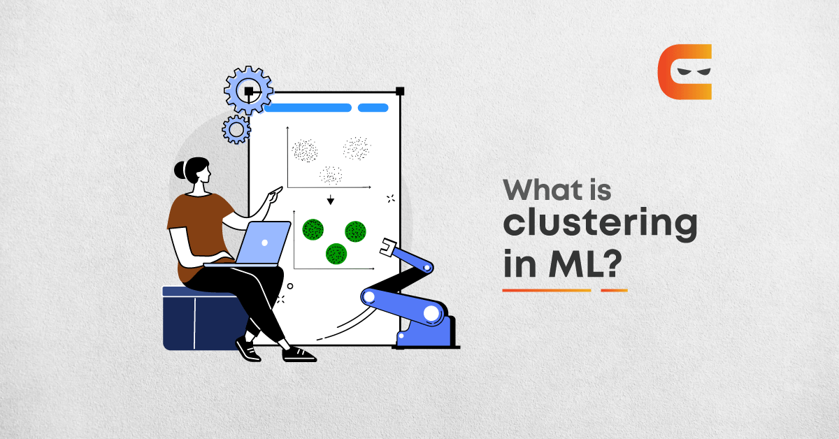
In simple terms, if we can group objects in our surroundings that share some common traits or say – “Correlated,” it is a cluster for us. Now, think of doing it with the data points from a vast dataset. If we can do the same thing with the data points by finding out some traits or patterns or a correlation, we can create clusters, can’t we? Well, that’s clustering in machine learning for you guys! Simple, isn’t it?

Types of Clustering in Machine Learning

We can divide clustering in machine learning broadly into two types:

• Hard Clustering: Hard clustering is about grouping the data items to existing strictly in one cluster. For example, we want the algorithm to read all of the tweets and determine if a tweet is a positive or a negative tweet.

• Soft Clustering: Soft Clustering is about grouping the data items to exist in multiple clusters. For example, if we want to categorize the items into fruits and vegetables, red and green apples fall into the fruit group; we can have them as two groups on other subcategories.

Clustering Models

Before jumping into the technicalities of clustering, let me try to help you understand the idea behind clustering or grouping the objects.

When we say data points are correlated, share the same pattern, or even similar, what do we mean? This is something that we should always ask ourselves. So let me try to make these terms clear to you to relate to them when we use them next time.

We know that shirts can be categorized into multiple subcategories. The most trivial would be casual and formal subcategories. If I ask you to categorise the shirts from a pile into these two categories, I am sure you will be able to do so. Don’t you? Why is it so?

We as humans understand that there are some distinct characteristics based on which we can distinguish a shirt into these two subcategories. One of the typical traits or characteristics would be the collar button.

There could be numerous traits on which we can differentiate; this is the idea I want to sow in your brains! Now, representing a “data point” for a shirt to carry out such analysis is another discussion covering a separate blog.

In a nutshell, the likeness or correlation among the data points may differ based on the end goals for a given dataset.

Clustering is one of the most frequently utilized forms of unsupervised learning, and we have 100’s of algorithms to categorize the data. But few of them are very popular and are used by most data-driven companies and startups. So let’s have a look at them in detail.

• Connectivity Models: This can also be called “Hierarchical Clustering.” The endpoint of the algorithm is a bunch of groups, where each bunch is distinct from one another. The items inside each group are correlated to another. So if they have the same patterns, they will fall under one group.

Hierarchical Clustering generally falls into two types (not discussed in detail in this blog):

• Agglomerative: This is a “bottom-up” approach – each observation starts in its cluster, and pairs of clusters are merged as one moves up the hierarchy.
• Divisive: This is a “top-down” approach – all observations start in one cluster, and splits are performed recursively as one moves down the hierarchy.

Image Source: Towards Data Science

Ex: The data is from US Twitter users during their elections. We can categorize the data: Reds are Republicans; Blues are Democrats; Blacks are independent. As you can see, Democrats and Republicans are very clearly split from the top, showing the success of this method. We just categorized the data based on people supporting their respective parties.

• Centroid models: These are iterative clustering algorithms in which the idea of likeness is determined by the closeness of information that highlights the centroid of the groups. In these models, the number of clusters needed toward the end must be referenced initially.
  • Ex: This model has one of the most famous algorithms that is K-Means clustering. This algorithm intends to segment n perceptions into K-Means clustering in which every perception has a place with the group with the closest mean, filling in as a model of the bunch.

• Distribution Models: These are iterative clustering algorithms in which the idea of likeness is to determine by the closeness of information highlight the centroid of the groups. In these models, the number of clusters needed toward the end must be referenced in the beginning.
  • Ex: A famous illustration of these models is the Expectation-Maximisation algorithm which utilizes multivariate normal distributions.

• Density models: These models search the information space for areas of data points of data space. It secludes different diverse density areas and allocates the data points inside these locales in a similar group.
  • Ex:  Mainstream instances of thickness models are Density-Based Spatial Clustering of Applications with Noise (DBSCAN) and Oscura Peak tracker Investigation and Comparison Series (OPTICS).

We have tons of algorithms based on the above models, but in this blog, we will cover three of the famous algorithms. We will also look at their implementation in Python. Using a jupyter notebook to run the code snippets is highly recommended.

Clustering Algorithms

We will be using the iris dataset (you can read the official documentation here) to implement the clustering algorithms and see how the clustering algorithms behave differently when applied to the same dataset.

1. K-Means Clustering:

K Means Clustering algorithm is an iterative algorithm that aims to find the local maxima in each iteration. We can solve this problem in five steps:

• Let’s take a variable named ‘K,’ which means the count of whole clusters. 2First, you need to specify the desired number of groups. Let choose the K=2 and 5 data points in a 2-D space. The below diagram shows the visualization of the 2 clusters and 5 data points.

• The centroid for red data points can be marked as the red cross, and the grey data points centroid is marked with a grey cross mark.

• Now let’s rearrange the data points. The bottom one is assigned to the grey cluster because it is close to the grey cross mark.

• Now let’s recompute the centroids for both the red and grey clusters.
• Recompute the centroids for both clusters.

Note: Repeat steps 4,5 until no improvements are possible. We repeat the steps until we reach global optima. A globally optimal solution is a feasible solution with an objective value that is as good or better than all other feasible solutions to the model. When there is no switching of data points between clusters, it is marked as the termination of the algorithm.

Image source: Javapoint.com

The above picture describes how data is segregated while we use the K-Means algorithm. The complete information is grouped into three different groups as they are grouped based on the centroid.

Code:

from matplotlib import pyplot as plt
from sklearn import datasets
from numpy import unique
from numpy import where
from sklearn.cluster import KMeans

# import some data to play with
iris = datasets.load_iris()
x = iris.data[:, :2]  # we only take the first two features sepal length and sepal width respectively.

model = KMeans(n_clusters = 3)
yhat = model.fit_predict(x)

# retrieve unique clusters
clusters = unique(yhat)

# create scatter plot for samples from each cluster
for cluster in clusters:
	# get row indexes for samples with this cluster
	row_ix = where(yhat == cluster)
	# create scatter of these samples
	plt.scatter(x[row_ix, 0], x[row_ix, 1])

    
plt.xlabel('Sepal length')
plt.ylabel('Sepal width') 

# show the plot
plt.show()


Output:

Since we knew that the dataset can be classified into three distinct clusters, we could initialise the k = 3. 
The plot is against the sepal width and sepal length. It gives us an insight to the data points as from where they have split and defines the boundaries for every cluster.
We need to note that varying k will result in different numbers of clusters.

Advantages of K-Means Clustering

• This algorithm can be applied to any form of data where the data has numerical entities.
• It is much faster than other algorithms.
• It is easy to interpret and understand.
• It guarantees convergence.
• We can generalise clusters, different shapes, and graphs.
• It can quickly adapt to new examples or new data.

Disadvantages of K-Means Clustering

• K-Means Clustering algorithm fails for non-linear data.
• At the start of the algorithm, the user must give the number of clusters, so sometimes groups may be more or less to solve.
• This algorithm doesn’t work for categorical data.
• It cannot handle outliers.

2. DBSCAN (Density-Based Spatial Clustering of Applications with Noise) Algorithm

DBSCAN is a well-known algorithm for machine learning and data mining. The DBSCAN algorithm can find associations and structures in data that are hard to find manually but can be relevant and helpful in finding patterns and predicting trends.

Ex: DBSCAN algorithm is used in many applications of maths and sciences. The best example is e-commerce website recommendations. For instance, customer X has brought one sanitiser bottle and five face masks.

However, customer Y had brought only one sanitiser bottle, so the algorithm recommends the face masks to customer Y because it is the most bought item.

Image Source: Amazon

The DBSCAN algorithm requires only two parameters. To choose suitable parameters, we need to understand how they are used and have basic knowledge about the dataset.

• eps: It specifies how points should be closer to each other. If eps is chosen too small, a large part of the data will not be clustered. On the other hand, if large values are chosen, clusters will get merged. The value should be based on the distance of the dataset. In general, small values are preferable.

• minPoints: The minimum number of points to form a dense region is called minPoints.
  • Ex: If the goal is set at 5 points, we need at least 5 points to form a dense region.
  • The minimum value for minPoints is 3, but the more significant the dataset, the larger the minPoints value that should be chosen. This is because larger values are better for datasets with noise and will form more efficiently.

Code:

# DBSCAN clustering
from matplotlib import pyplot as plt
from sklearn import datasets
from numpy import unique
from numpy import where
from sklearn.cluster import DBSCAN

# import some data to play with
iris = datasets.load_iris()
x = iris.data[:, :2]  # we only take the first two features sepal length and sepal width respectively.

model = DBSCAN(eps = 0.4, min_samples = 9)
yhat = model.fit_predict(x)

# retrieve unique clusters
clusters = unique(yhat)

# create scatter plot for samples from each cluster
for cluster in clusters:
	# get row indexes for samples with this cluster
	row_ix = where(yhat == cluster)
	# create scatter of these samples
	plt.scatter(x[row_ix, 0], x[row_ix, 1])

    
plt.xlabel('Sepal length')
plt.ylabel('Sepal width') 

# show the plot
plt.show()


Output:

We are viewing a scatter plot for the same iris dataset on which we applied the k-means algorithm. Here we see a different picture altogether in terms of the clusters DBSCAN created.

If you play around with the parameters(eps and min_samlples) you get to see something else! It is very important to choose the algorithms depending on the use case and the kind of data we are trying to work upon.

Advantages of DBSCAN

•  Does not require a prior specification of several clusters.
• Able to identify noise data while clustering.
• The DBSCAN algorithm can find arbitrarily sized and arbitrarily shaped clusters.

Disadvantages of DBSCAN

• The DBSCAN algorithm fails in the case of varying density clusters.
• Fails in case of neck type of dataset.

• Mean Shift Algorithm:

Mean shift is also one of the clustering algorithms which involves finding and adapting centroids based on the density of examples in the feature space. The mean shift algorithm seeks modes or local maxima of density in feature spaces.

Ex: The mean shift algorithm is used for photography, filming. The mean shift algorithm converts a picture into pixels on a 3-D axis.

Image source: Mathworks.com

When the parrot image is given as an input picture, it is converted into pixel distribution on a 3-D axis.

To implement the Mean shift algorithm, we need only four basic steps:

• First, start with the data points assigned to a cluster of their own.
• Second, calculate the mean for all points in the window.

• Third, move the center of the window to the location of the mean.
• Finally, repeat steps 2,3 until there is a convergence.

Code:

# mean shift clustering
from matplotlib import pyplot as plt
from sklearn import datasets
from numpy import unique
from numpy import where
from sklearn.cluster import MeanShift

# import some data to play with
iris = datasets.load_iris()
x = iris.data[:, :2]  # we only take the first two features sepal length and sepal width respectively.

# define the model
model = MeanShift()

# fit model and predict clusters
yhat = model.fit_predict(x)

# retrieve unique clusters
clusters = unique(yhat)

# create scatter plot for samples from each cluster
for cluster in clusters:
	# get row indexes for samples with this cluster
	row_ix = where(yhat == cluster)
	# create scatter of these samples
	plt.scatter(x[row_ix, 0], x[row_ix, 1])

plt.xlabel('Sepal length')
plt.ylabel('Sepal width')

# show the plot
plt.show()


Output:

Comparing the clusters formed upon applying the mean shift algorithm to the initial one, k-means, we see that the clusters have made justice, though it could deduce two clusters. We don't have the leverage to tweak the number of clusters in the mean shift. 

Advantages of Mean Shift Algorithm

• The mean shift algorithm has only one parameter, which determines the number of clusters.
• There is no issue of local maxima and assumptions of total clusters.
• It also models the complex-shaped clusters.

Disadvantages of Mean Shift Algorithm

• The mean shift algorithm doesn’t work in the case of high dimension, where clusters change abruptly.
• We cannot have direct control over the number of clusters.

We saw how different clustering algorithms are applied on the same dataset. You would now have an idea of how difficult it could get while choosing the right algorithm for your use case. Diving deep into the data to see what others can’t will lead you in the race! 

Applications of Clustering

Clustering has vast applications in different fields. So some of the popular applications are:

• It can provide recommendations, like Netflix Movie suggestions.
• Sales or Marketing analysis
• Medical Image Analysis
• Anomaly detection
• Pattern Recognition
• Document classification

Frequently Asked Questions

Key Takeaways

In this article, we discussed what clustering means, its types, and types of clustering algorithms. Then we had a brief overview of K-Means clustering, DBSCAN, and Mean Shift algorithm. We also discussed each algorithms’ advantages and disadvantages along with the sample code for each one of them.

By Dharani Mandla