Depth-first search (DFS) is popularly known to be an algorithm for traversing or searching tree or graph data structures. The algorithm starts at the basis node (selecting some arbitrary node because the root node within the case of a graph) and explores as far as possible along each branch before backtracking.
A version of the depth-first search was investigated prominently in the 19th century by French mathematician Charles Pierre Trémaux as a technique for solving mazes.
For the following graph here, drawn below:
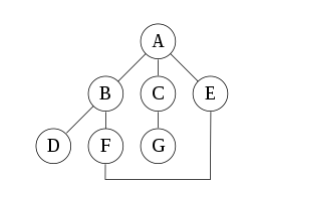
An undirected graph with edges AB, BD, BF, FE, AC, CG, AE is stated. A depth-first search starting at A, assuming that the left edges within the shown graph are chosen before right edges, and assuming the search remembers previously visited nodes and can not repeat them (since this is a small graph), will visit the nodes in the following order: A, B, D, F, E, C, G. The edges traversed during this search form a Trémaux tree, a structure with important applications in graph theory. Performing an equivalent search without remembering previously visited nodes leads to visiting nodes within the order A, B, D, F, E, A, B, D, F, E, etc. forever, caught within the A, B, D, F, E cycle and never reaching C or G.
Iterative deepening, as we know it is one technique to avoid this infinite loop and would reach all nodes. A convenient description of a depth-first search (DFS) of a graph is in terms of a spanning tree of the vertices reached during the search, which is one theory that can be explained well with graphs. Based on this spanning tree, the sides of the first graph are often divided into three classes: forward edges, which point from a node of the tree to at least one of its descendants, back edges, which point from a node to at least one of its ancestors, and cross edges, which do neither.
Sometimes tree edges, edges which belong to the spanning tree itself, are classified separately from forwarding edges and it’s a fact that if the first graph is undirected then all of its edges are tree edges or back edges.
DFS Ordering: An enumeration of the vertices of a graph is said to be a DFS order if it is the possible output of the application of DFS to this graph.
Vertex Ordering: It is also very much possible as it has been proved that we can use depth-first search to linearly order the vertices of a graph or tree. There are four possible ways of doing this: A preordering may be a list of the vertices within the order that they were first visited by the depth-first search algorithm. this is often a compact and natural way of describing the progress of the search, as was done earlier during this article. A preordering of an expression tree is that the expression in prefix notation.
A post-order may be a list of the vertices within the order that they were last visited by the algorithm. A post ordering of an expression tree is that the expression in reverse prefix notation.
A reverse preordering is that the reverse of a preordering, i.e. an inventory of the vertices within the opposite order of their first visit. Reverse preordering isn’t an equivalent as post ordering. A reverse post ordering is that the reverse of a post order, i.e. an inventory of the vertices within the opposite order of their last visit.
Reverse post ordering isn’t an equivalent as preordering. For binary trees, there’s additionally in-ordering and reverse in-ordering.
For example, when searching the directed graph below beginning at node A, the sequence of traversals, known to us is either A B D B A C A or A C D C A B A (choosing to first visit B or C from A is up to the algorithm). Note that repeat visits within the sort of backtracking to a node, to see if it’s still unvisited neighbours, are included here (even if it’s found to possess none). Thus the possible pre-ordering is A B D C and A C D B, while the possible post-orderings are D B C A and D C B A, and therefore the possible reverse post-orderings are A C B D and A B C D, which will also help in the future to show the implementation of DFS by an adjacency matrix.
What is an adjacency matrix?
In graph theory and computing, an adjacency matrix may be a matrix wont to represent a finite graph. the weather of the matrix indicates whether pairs of vertices are adjacent or not within the graph. In the special case of a finite simple graph, the adjacency matrix may be a (0,1)-matrix with zeros on its diagonal. If the graph is undirected (i.e. all of its edges are bidirectional), the adjacency matrix is symmetric. the connection between a graph and therefore the eigenvalues and eigenvectors of its adjacency matrix is studied in spectral graph theory.
The adjacency matrix of a graph should be distinguished from its incidence matrix, a special matrix representation whose elements indicate whether vertex–edge pairs are incident or not, and its degree matrix, which contains information about the degree of every vertex.
Definition:
For an easy graph with vertex set V, the adjacency matrix may be a square |V| × |V| matrix A such its element Aij is one when there’s a foothold from vertex I to vertex j, and 0 when there’s no edge.[1] The
diagonal elements of the matrix are all zero since edges from a vertex to itself (loops) aren’t allowed in simple graphs. it’s also sometimes useful in algebraic graph theory to exchange the nonzero elements with
algebraic variables.
An equivalent concept is often extended to multigraphs and graphs with loops by storing the number of edges between every two vertices within the corresponding matrix element and by allowing nonzero diagonal elements. Loops could also be counted either once (as one edge) or twice (as two vertex-edge incidences), as long as a uniform convention is followed. Undirected graphs often use the latter convention of counting loops twice, whereas directed graphs typically use the previous convention.
Data Structures: The adjacency matrix could also be used as a knowledge structure for the representation of graphs in computer programs for manipulating graphs. the most alternative arrangement, also in use for this application, is that the adjacency list.
Because each entry within the adjacency matrix requires just one bit, it is often represented during a very compact way, occupying only |V|2/8 bytes to represent a directed graph, or (by employing a packed
triangular format and only storing the lower triangular a part of the matrix) approximately |V|2/16 bytes to represent an undirected graph.
Examples:
Undirected Graphs: The convention followed here (for undirected graphs) is that every edge adds 1 to the acceptable cell within the matrix, and every loop adds 2.[4] this enables the degree of a vertex to be easily found by taking the sum of the values in either its respective row or column within the adjacency
matrix.
Directed Graphs: The adjacency matrix of a directed graph are often asymmetric. One can define the adjacency matrix of a directed graph either such:
- A non-zero element Aij indicates a foothold from i to j or
- It indicates a foothold from j to i
Trivial Graphs: The adjacency matrix of an entire graph contains all ones except along the diagonal where there are only zeros. The adjacency matrix of an empty graph may be a zero matrix.
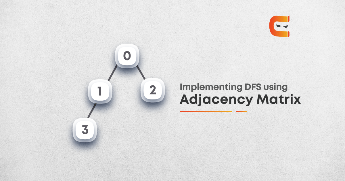
Implementation of DFS using adjacency matrix
Depth First Search (DFS) has been discussed before as well which uses adjacency list for the graph representation. Now in this section, the adjacency matrix will be used to represent the graph.
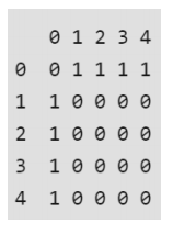
Adjacency matrix representation: In adjacency matrix representation of a graph, the matrix mat[][] of size n*n (where n is the number of vertices) will represent the edges of the graph where mat[i][j] = 1 represents that there is an edge between the vertices i and j while mat[i][i] = 0 represents that there is no edge between the vertices i and j. Just consider the image as an example.
Below is the adjacency matrix representation of the graph shown in the above image:
Approach that we will be following:
- Create a matrix of size n*n where every element is 0 representing there is no edge in the graph.
- Now, for every edge of the graph between the vertices i and j set mat[i][j] = 1.
- After the adjacency matrix has been created and filled, call the recursive function for the source i.e. vertex 0 that will recursively call the same function for all the vertices adjacent to it.
- Also, keep an array to keep track of the visited vertices that are shown as: visited[i] = true represents that vertex I have been visited before and the DFS function for some already visited node need not be called.
Depth-first search(DFS): DFS is traversing or searching tree or graph data structures algorithm. The algorithm starts at the root node and explores as far as possible or we find the goal node or the node which has no children. It then backtracks from the dead-end towards the most recent node that is yet to be completely unexplored. DFS uses Depth wise searching. DFS data structure uses the stack. In DFS, the sides that results in an unvisited node are called discovery edges while the sides that results in an already visited node are called block edges.
Steps for searching:
- Push the root node in the stack.
- Loop until the stack is empty.
- Peek the node of the stack.
- If the node has unvisited child nodes, get the unvisited child node, mark it as traversed and push it on the stack.
- If the node does not have any unvisited child nodes, pop the node from the stack.
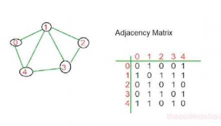
Adjacency Matrix: it’s a two-dimensional array with Boolean flags. As an example, we will represent the sides for the above graph using the subsequent adjacency matrix.
- n by n matrix, where n is number of vertices
- A[m,n] = 1 iff (m,n) is an edge, or 0 otherwise
- For weighted graph: A[m,n] = w (weight of edge), or positive infinity otherwise
Advantages of Adjacency Matrix:
- Adjacency matrix representation of the graph is very simple to implement
- Adding or removing time of an edge can be done in O(1) time. Same time is required to check if there is an edge between two vertices
- It is very convenient and simple to programme
Disadvantages of Adjacency Matrix:
- It consumes a huge amount of memory for storing big graphs
- It requires huge efforts for adding or removing a vertex. If you are constructing a graph in dynamic structure, the adjacency matrix is quite slow for big graphs
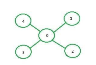
Example:
from the above graph in the picture the path is
0—–>1—–>2—–>3—–>4
Programme:
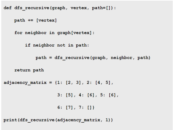
Output: [1, 2, 4, 6, 7, 5, 3]
To explore more articles, click here.
By Deepak Jain


