A regression model is basically a representation of a set of independent quantity on a unit dependent quantity, that dependent quantity in machine learning is our output value produced from the set of input that is independent values or records.
In the graphical representation of 2D data, we represent our X-axis as a set of independent values and Y-axis as the outcome or the dependent value.
Need for Regression
The two main reasons of using regression are:
- It is mostly used in prediction, which is part of the machine learning technique.
- It may also be used in the representation of the relationship between independent and dependent data.
There are mainly six types of Regression models used according to the requirement of different format of data available to us.
All the six models are the part of sklearn.linear_model library of sklearn,
- Linear Regression
- Logistic Regression
- Ridge Regression
- Lasso Regression
- Polynomial Regression
- Bayesian Linear Regression
Linear Regression and Logistic Regression are the two main regression model used in many cases or different type of dataset but apart from that four other regression model can also be used depending upon the requirements and factors involved.
Detail description of each model is given below:
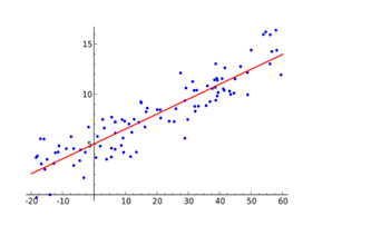
Linear Regression: This regression model is the most common one among all the models available, this model focus on fitting the set of dependent and independent dataset in a linear line function, an equation for the representation of a linear function is mentioned below:
y = mx + b
where y is our output data, x is the independent data, m is slope, b is intercept.
Linear regression assumes the linear relationship between set of independent and dependent data sets. If we have more than one independent variable or set of independent variables as
X = {x1, x2, x3, …… , xn}
then the linear regression model is known as multiple linear regression.
Equation for representation of multiple linear regression is
y = m1x1 + m2x2 + m3x3 + …… + mnxn + b
for the set of n independent variables.
This model focus on minimization of error between each point on the line.
In order to use the linear regression model, we need to import it as,
from sklearn.linear_model import LinearRegression
this will import LinearRegression in our file, we need to create an object of LinearRegression model as,
alg = LinearRegression( )
alg is the main object that will be used for further processing to fit the data in linear function and for the final prediction of output.
Logistic Regression: Another most common type of regression model is Logistic regression model, this is mostly used when the data is in a discrete format which is it either in the format of 0/1 or true/false, here the dependent value is in discrete format and the independent data should not have any correlation between them.
Logistic regression tries to find the best boundary line in order to fit the data according to the format, this type of regression mostly used when the data is present in a large amount. The relationship between dependent and independent values is expressed by the sigmoid curve, an equation that denotes the logistic regression is:
y = 1/(1 + e-z)
here y is our discrete dependent variable and z is linear representation of set of independent variables as,
z = mx + c
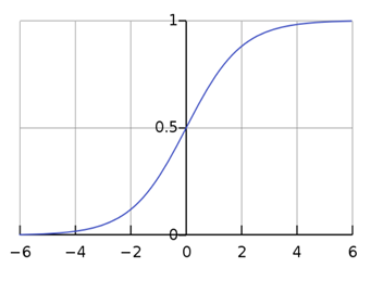
on the bases of the equation, we can predict the value as 0/1 for example,
if z > 0 then y > 0.5, in that case, the result may be predicted as 1
OR
if z < = 0 then y <= 0.5 this may lead to of prediction of 0
these conditions can be vice-versa depending upon the behaviour of output.
Logistic regression can also be imported from sklearn.linear_model and can be used by declaring an object for logistic regression.
Ridge Regression: This type of regression is mostly used when we have highly correlated data that is the independent set of data have a very strong relationship among each other, this can be seen as the advance version of linear regression as we include the bias in our expression in order to reduce the standard errors due to multicollinearity. In multicollinearity we have high value of variances which moves the prediction value far away from true value.
Normal equation that we use in case of linear regression:
y = mx + b
in case of ridge regression model, we have:
y = mx + b + e
where: y is our output or dependent value, x is independent value, b is intercept and e is our bias used to reduce the standard error.
In case of multiple independent variables, we have:
y = m1x1 + m2x2 + m3x3 + …… + mnxn + b + e
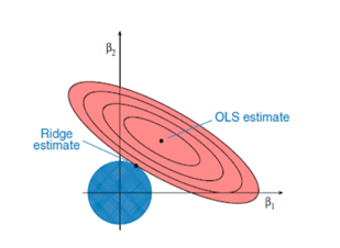
the problem of multicollinearity is solved using shrinkage parameter (lambda) which is added to the least square error value in order to reduce the value of variance,
error = |y – (mx + b)|2 + (lambda)|mx+b|2
ridge regression tries to put the points in a such a way that value of the coefficients shrinks but doesn’t reaches zero.
Lasso Regression: Lasso stand for least absolute shrinkage and selection operator, this regression model is mostly similar to ridge regression model except it use the absolute value in error function rather than using square value, which in turn reduces the large change in variance and increase the accuracy of linear regression model,
error = |y – (mx + b)|2 + (lambda)|mx+b|
this may cause penalising values which lead to estimation of exactly zero for some of the parameters.
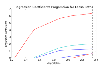
It can be said that lasso regression performs regularisation along with feature selection that is, it selects out an only certain set of features from the total set of features that will be given as the input to the model, in that case only the needed features are used up and all the other unrequired features are made to be zero and hence save the model from over-fitting.
Polynomial Regression: This model is nearly same as linear regression model with certain degree attach to it, with a certain degree it means, the relationship between the dependent and independent values (or the set) is not linear, it may change with a degree of 2, 3, 4 or so on. The typical equation to represent the polynomial regression is:
y = ax2 + b
here: y is dependent on square power of x
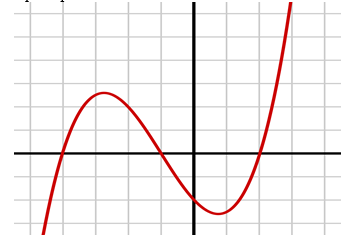
In polynomial regression the line or curve passes from each data points depending on degree of variation. This model sometimes may lead to over-fitting because mean squared error tries to minimise the error in order to the best fit curve/line that is why typical analysation is required to use this model.
Bayesian Linear Regression: This regression model uses the Bayes theorem to obtain the value of regression coefficients that are using probability distributions, Bayesian Linear Regression is the combination of both linear and Ridge Regression but it is more stable than simple linear regression. The main goal of this regression model is to determine the posterior distribution for the model.
This regression model uses the Bayes theorem to obtain the value of regression coefficients that are using probability distributions, Bayesian Linear Regression is the combination of both linear and Ridge Regression but it is more stable than simple linear regression. The main goal of this regression model is to determine the posterior distribution for the model.
To explore more about Machine Learning, click here.
By Vikas Upadhyay


