Before we hop into the derivation of simple linear regression, it’s important for us to have a very strong intuition on what we are actually going to do and especially why we are going to do it? With that being said, let’s dive in!
What is Regression?
Regression analysis is a set of statistical approaches that are used to determine the relationships between the dependent variable(output) and the independent variable(input).
What is an Independent Variable?
Independent variable is also called an input variable. If we want to create a machine learning model then we must have some dataset, based on which we will predict the value of output. So, the variables in the dataset which we are going to use to build a model are called independent variables.
What is the Dependent Variable?
The dependent variable is also called the output variable. We build machine learning models to predict a variable based on the input data. So here we can say that the output variable is dependent on the input data, that’s why it’s called a dependent variable.
Simple Linear Regression:
To see when we are going to need to use Simple Linear Regression, why don’t we start with a story of some friends!
Let’s say there lived some friends named SpongeBob, Patrick, Squidward and Gary in the “Bikini Bottom!”. One day Squidward went to SpongeBob and had this conversation. Let’s check it out.
Squidward: “Hey SpongeBob I’ve heard you’re so smart!”
SpongeBob: “Yes sir! There is no doubt in that.”
Squidward: “Is that so?”
SpongeBob: “Umm..Yes…”
Squidward: “So here’s the thing.. I want to sell my house as I’m going to shift to my new lavish house in downtown. But I can’t figure out at which price I should sell my house! If I keep the price too high then no one is going to buy it and if I set the price low then I might face tremendous financial loss! So you have to help me find the best price for my house. But keep in mind you have only one day!”
(SpongeBob is stressed as always but he’s very optimistic about finding the solution. To discuss the problem he went to his shrewd friend Patrick’s house.)
(Patrick is in his living room watching TV with a big bowl of popcorn in his hands.)
(SpongeBob described the whole situation to Patrick.)
Patrick: “That’s a piece of cake, my friend! Follow me!”
(They decided to go to Squidward’s neighbourhood, where his two neighbours recently sold their houses. After some time they were able to find out the square footage and selling price of their houses.)
Here’s the dug data!
House A:
Area = 1500 ft.
Price = 150000$
House B:
Area = 2500 ft.
Price = 300000$
Now here notice that the actual price of the house is dependent on various factors like:
- Area
- Neighbourhood
- Time of Year
- Demand
- Location
But since this is simple linear regression and it’s the first tutorial so we are just going to consider the area of the house as an independent variable to calculate the price of the dependent variable price of the house.
(From the collected data Patrick was able to draw the following graph.)
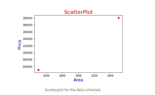
Now after pensive thinking Patrick was able to predict the selling price for Squidward’s house. Here’s an explanation provided by him. When we have two given points in a coordinate plane we can always find the equation of line passing through the two points.
Here’s the formula for that :
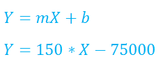
Y=mX + b (Equation of Line)
Where,
m = Slope of the line
b = Y — intercept of the line
Y = Y — coordinate of the point from which line passes through
X = X — coordinate of the point from which line passes through
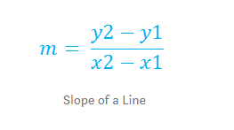
What is the slope of a line?
To understand it much better let’s see some basics on coordinate geometry.
Basics of coordinate geometry:
Some rules for choosing the points in the coordinate plane:
(1) We always look from left to right in the coordinate plane to name the points.
(2) After looking from left-to-right, the first point we get must be named (x1,y1) and the second point will be (x2,y2).
(3) Horizontal lines have a slope of 0.
(4) Vertical lines have “Infinite” slope.
(5) If the Y-coordinate of the second point is greater than the Y-coordinate of the first point then the line has positive(+) slope, else the line has a negative slope.
(6) Points at the same vertical distance from X-axis have same Y-coordinate.
(7) Points at the same vertical distance from Y-axis have the same X-coordinate.
So, from the above mentioned rules we can say that in our graph :
(x1,y1) = ( 1500,150000)
(x2,y2) = (2500,300000)
Now we can easily find the slope:

Now since we want to predict the value of Y, we must have values of X, m , b. Next, we are going to find the value of intercept b. Notice that we already have values of X and m, so after finding the value of b, we will be able to actually predict the output variable.
Now since we have all the other values, we can calculate the value of slope b.
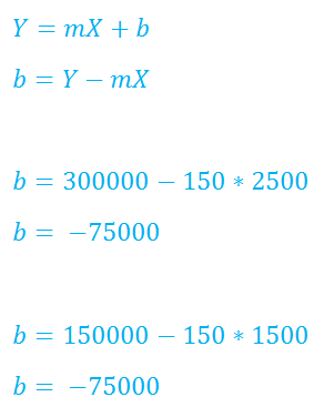
Now we have our finalised equation of slope:
(Now Patrick and SpongeBob went to Squidward to find out the square footage of his house.)
SpongeBob: “Hey Squidward, can you tell me the total area in square footage of your house?”
Squidward: “Whyyy?”
SpongeBob: “Do you want to sell your house or not?”
Squidward: “Okay..Okay..It’s 1800 square feets.”
(SpongeBob and Patrick left the store.)
Now, in our equation :
Y : Price of house
X : Area in square feets
Now, putting the value of the area of squidward’s house :
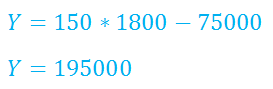
Now, we can say that squidward should sell his house for 195000$.
(Now SpongeBob and Patrick decided to their another ingenious friend Gary the snail for confirmation of the number that they predicted.)
SpongeBob: “Hey Gary, can you confirm that the prices we predicted for Squidward’s house are correct?”
Gary: (Meditating for a minute) “I think you are underpricing the house.”
SpongeBob: “Butttt….!”
Patrick: “Can you help us?”
(Gary holds him a paper that has data about 100 houses in the city with it’s price and area.)
(SpongeBob and Patrick went home and plotted the data on the coordinate plane.)
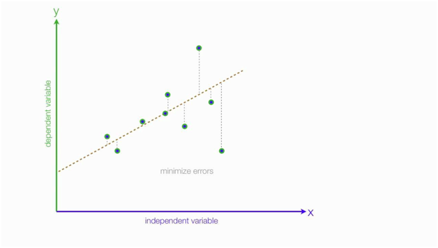
Now, here we can see that using two points to plot a line won’t work in this situation, we must find a line that “best fits” the 100 data points. When thinking about the best fit line — think one line that is closest to all the points. Instead of trial and error, we can determine this best fit by minimising a thing called the sum of squared errors.
Now what does it mean by “best fit” ?
As we can see in the graph that we can not plot a single straight line that passes through all the points. So what we can do here is to minimise the error. It means that we find a line and then find the error in prediction. Since we have the actual value here, we can easily find the error in prediction. Our ultimate goal will be to find the line that has the least error. That line is called the line that best fits the data.
Now there are many different methods to calculate the error. We’ll see some of them in later videos. Here we are going to use the Sum of Squared method to calculate the error. Let’s understand it in detail.
Sum of Squared Error:
To begin, we need to find an equation of a line that minimises the distance between all the data points we have plotted.
When asked about the explanation for Sum of Squared Error, Patrick explained the following :
One way to measure distance between the scattered points and the line is to find the distance between their Y values.
Let’s say we use our line from earlier : Y = 150X — 75000 and want to see how accurate our previous function is for a 1800 square foot house that actually sold for $220,000. Well if we input a 1800 square feet in our equation,it says we should have sold the house for $195,000, but in reality it sold for $220000. A difference of $25000. Point one for Gary!
In brief,
Actual selling price : $220,000
Predicted selling price : $195,000
Error in prediction : 220,000–195,000 = $25,000
This difference, or error, in price is exactly what we need to do for the rest of the 99 data points. Once we do this for each point, we then add the errors together to measure our accuracy. More formally stated…

and to account for negative numbers, we square the errors:

Now what we have to do is find the error for all of the data points and add it. First, we’ll try it for one line and calculate the error, after then we are going to update the parameters of the lines and then again find the error and we’ll continue this until we find the best fit line.
Don’t worry we’re not going to do this manually, we’ll use python code to implement it. But it’s always good to know how it works internally. Now what we have to do is to minimise this error to predict the output price more accurately. Well, we can say that once they are equipped with that power we’ll be able to predict the house price of almost every house in our neighbourhood.
Guidelines for regression line:
- Use regression lines when there is a significant correlation to predict values.
- Stay within the range of the data. Do not extrapolate!! For example, if the data is from 10 to 60 don’t try to predict the value for 500.
- Don’t make a prediction for a population-based on another population’s regression line.
Use-case of linear regression:
- Height and weight
- Alcohol consumed and blood alcohol content
- Vital lung capacity and pack-years of smoking
- Driving speed and gas mileage
Moving forward, in the next part we’ll see about brute force attack to get the value of slope and intercept for our “best-fit” line.
Special thanks to : Patrick , SpongeBob ,Gary , Squidward! 🙂

To learn more about Liner Regression, click here.
By Pratik Shukla


